Apart from training/testing scripts, We provide lots of useful tools under the
tools/ directory.
Log Analysis
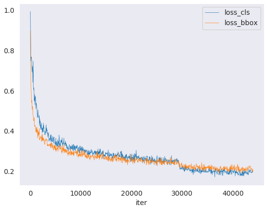
tools/analysis_tools/analyze_logs.py plots loss/mAP curves given a training
log file. Run pip install seaborn first to install the dependency.
python tools/analysis_tools/analyze_logs.py plot_curve [--keys ${KEYS}] [--title ${TITLE}] [--legend ${LEGEND}] [--backend ${BACKEND}] [--style ${STYLE}] [--out ${OUT_FILE}]
Examples:
Plot the classification loss of some run.
python tools/analysis_tools/analyze_logs.py plot_curve log.json --keys loss_cls --legend loss_cls
Plot the classification and regression loss of some run, and save the figure to a pdf.
python tools/analysis_tools/analyze_logs.py plot_curve log.json --keys loss_cls loss_bbox --out losses.pdf
Compare the bbox mAP of two runs in the same figure.
python tools/analysis_tools/analyze_logs.py plot_curve log1.json log2.json --keys bbox_mAP --legend run1 run2
Compute the average training speed.
python tools/analysis_tools/analyze_logs.py cal_train_time log.json [--include-outliers]
The output is expected to be like the following.
-----Analyze train time of work_dirs/some_exp/20190611_192040.log.json-----
slowest epoch 11, average time is 1.2024
fastest epoch 1, average time is 1.1909
time std over epochs is 0.0028
average iter time: 1.1959 s/iter
Visualization
Visualize Datasets
tools/misc/browse_dataset.py helps the user to browse a detection dataset (both
images and bounding box annotations) visually, or save the image to a
designated directory.
python tools/misc/browse_dataset.py ${CONFIG} [-h] [--skip-type ${SKIP_TYPE[SKIP_TYPE...]}] [--output-dir ${OUTPUT_DIR}] [--not-show] [--show-interval ${SHOW_INTERVAL}]
Model Serving
In order to serve an MMRotate model with TorchServe, you can follow the steps:
1. Convert model from MMRotate to TorchServe
python tools/deployment/mmrotate2torchserve.py ${CONFIG_FILE} ${CHECKPOINT_FILE} \
--output-folder ${MODEL_STORE} \
--model-name ${MODEL_NAME}
Example:
wget -P checkpoint  \
https://download.openmmlab.com/mmrotate/v0.1.0/rotated_faster_rcnn/rotated_faster_rcnn_r50_fpn_1x_dota_le90/rotated_faster_rcnn_r50_fpn_1x_dota_le90-0393aa5c.pth

python tools/deployment/mmrotate2torchserve.py configs/rotated_faster_rcnn/rotated_faster_rcnn_r50_fpn_1x_dota_le90.py checkpoint/rotated_faster_rcnn_r50_fpn_1x_dota_le90-0393aa5c.pth \
--output-folder ${MODEL_STORE} \
--model-name rotated_faster_rcnn
Note: ${MODEL_STORE} needs to be an absolute path to a folder.
2. Build mmrotate-serve docker image
docker build -t mmrotate-serve:latest docker/serve/
3. Run mmrotate-serve
Check the official docs for running TorchServe with docker.
In order to run in GPU, you need to install nvidia-docker. You can omit the --gpus argument in order to run in CPU.
Example:
docker run --rm \
--cpus 8 \
--gpus device=0 \
-p8080:8080 -p8081:8081 -p8082:8082 \
--mount type=bind,source=$MODEL_STORE,target=/home/model-server/model-store \
mmrotate-serve:latest
Read the docs about the Inference (8080), Management (8081) and Metrics (8082) APis
4. Test deployment
curl -O https://raw.githubusercontent.com/open-mmlab/mmrotate/main/demo/demo.jpg
curl http://127.0.0.1:8080/predictions/${MODEL_NAME} -T demo.jpg
You should obtain a response similar to:
[
  {
    "class_name": "small-vehicle",
    "bbox": [
      584.9473266601562,
      327.2749938964844,
      38.45665740966797,
      16.898427963256836,
      -0.7229751944541931
    ],
    "score": 0.9766026139259338
  },
  {
    "class_name": "small-vehicle",
    "bbox": [
      152.0239715576172,
      305.92572021484375,
      43.144744873046875,
      18.85024642944336,
      0.014928221702575684
    ],
    "score": 0.972826361656189
  },
  {
    "class_name": "large-vehicle",
    "bbox": [
      160.58056640625,
      437.3690185546875,
      55.6795654296875,
      19.31710433959961,
      0.007036328315734863
    ],
    "score": 0.888836681842804
  },
  {
    "class_name": "large-vehicle",
    "bbox": [
      666.2868041992188,
      1011.3961181640625,
      60.396209716796875,
      21.821645736694336,
      0.8549195528030396
    ],
    "score": 0.8240180015563965
  }
]
And you can use test_torchserver.py to compare result of torchserver and pytorch, and visualize them.
python tools/deployment/test_torchserver.py ${IMAGE_FILE} ${CONFIG_FILE} ${CHECKPOINT_FILE} ${MODEL_NAME}
[--inference-addr ${INFERENCE_ADDR}] [--device ${DEVICE}] [--score-thr ${SCORE_THR}]
Example:
python tools/deployment/test_torchserver.py \
demo/demo.jpg \
configs/rotated_faster_rcnn/rotated_faster_rcnn_r50_fpn_1x_dota_le90.py \
rotated_faster_rcnn_r50_fpn_1x_dota_le90-0393aa5c.pth \
rotated_fater_rcnn
Model Complexity
tools/analysis_tools/get_flops.py is a script adapted from flops-counter.pytorch to compute the FLOPs and params of a given model.
python tools/analysis_tools/get_flops.py ${CONFIG_FILE} [--shape ${INPUT_SHAPE}]
You will get the results like this.
==============================
Input shape: (3, 1024, 1024)
Flops: 215.92 GFLOPs
Params: 36.42 M
==============================
Note: This tool is still experimental and we do not guarantee that the number is absolutely correct. You may well use the result for simple comparisons, but double check it before you adopt it in technical reports or papers.
FLOPs are related to the input shape while parameters are not. The default input shape is (1, 3, 1024, 1024).
Some operators are not counted into FLOPs like DCN and custom operators. So models with dcn such as S2A-Net and RepPoints based model got wrong flops. Refer to
mmcv.cnn.get_model_complexity_info()for details.The FLOPs of two-stage detectors is dependent on the number of proposals.
Prepare a model for publishing
tools/model_converters/publish_model.py helps users to prepare their model for publishing.
Before you upload a model to AWS, you may want to
convert model weights to CPU tensors
delete the optimizer states and
compute the hash of the checkpoint file and append the hash id to the filename.
python tools/model_converters/publish_model.py ${INPUT_FILENAME} ${OUTPUT_FILENAME}
E.g.,
python tools/model_converters/publish_model.py work_dirs/rotated_faster_rcnn/latest.pth rotated_faster_rcnn_r50_fpn_1x_dota_le90_20190801.pth
The final output filename will be rotated_faster_rcnn_r50_fpn_1x_dota_le90_20190801-{hash id}.pth.
Benchmark
FPS Benchmark
tools/analysis_tools/benchmark.py helps users to calculate FPS. The FPS value includes model forward and post-processing. In order to get a more accurate value, currently only supports single GPU distributed startup mode.
python -m torch.distributed.launch --nproc_per_node=1 --master_port=${PORT} tools/analysis_tools/benchmark.py \
    ${CONFIG} \
    ${CHECKPOINT} \
    [--repeat-num ${REPEAT_NUM}] \
    [--max-iter ${MAX_ITER}] \
    [--log-interval ${LOG_INTERVAL}] \
    --launcher pytorch
Examples: Assuming that you have already downloaded the Rotated Faster R-CNN model checkpoint to the directory checkpoints/.
python -m torch.distributed.launch --nproc_per_node=1 --master_port=29500 tools/analysis_tools/benchmark.py \
       configs/rotated_faster_rcnn/rotated_faster_rcnn_r50_fpn_1x_dota_le90.py \
       checkpoints/rotated_faster_rcnn_r50_fpn_1x_dota_le90-0393aa5c.pth \
       --launcher pytorch
Miscellaneous
Print the entire config
tools/misc/print_config.py prints the whole config verbatim, expanding all its
imports.
python tools/misc/print_config.py ${CONFIG} [-h] [--options ${OPTIONS [OPTIONS...]}]
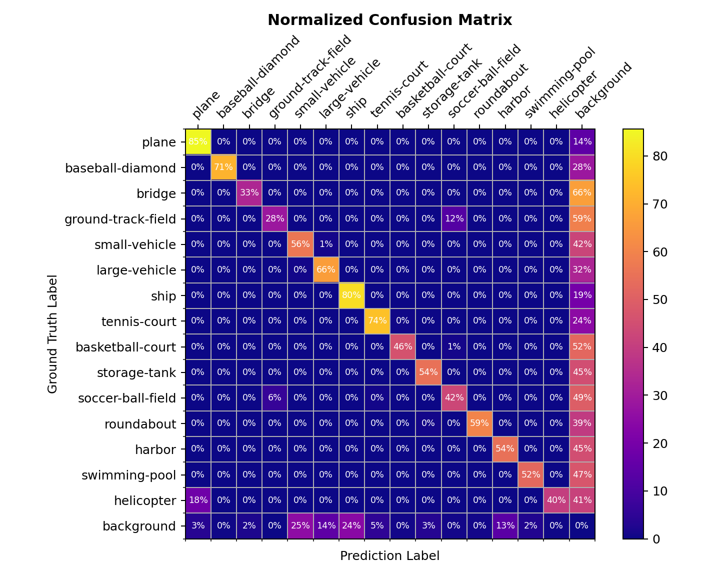
Confusion Matrix
A confusion matrix is a summary of prediction results.
tools/analysis_tools/confusion_matrix.py can analyze the prediction results and plot a confusion matrix table.
First, run tools/test.py to save the .pkl detection results.
Then, run
python tools/analysis_tools/confusion_matrix.py ${CONFIG} ${DETECTION_RESULTS} ${SAVE_DIR} --show
And you will get a confusion matrix like this: